Visualizing the Model
After building an AuroraModel, plot_model can be called to produce a set of diagnostic figures that let you inspect the atmosphere, energy grid, cross-sections, phase functions, and scattering data before running a simulation.
Quick start
using AURORA
using CairoMakie

altitude_lims = [100, 600]
θ_lims = 180:-10:0
E_max = 3000

msis_file = find_msis_file(year=2005, month=10, day=8, hour=22, minute=0,
                           lat=70, lon=19, height=85:1:700)
iri_file = find_iri_file(year=2005, month=10, day=8, hour=22, minute=0,
                         lat=70, lon=19, height=85:1:700)

model = AuroraModel(altitude_lims, θ_lims, E_max, msis_file, iri_file)
initialize!(model)   # build densities, cross-sections, phase functions, and scattering data
Looking for an msis file that matches the parameters... no file was found.
Calculating msis data... done.
File msis_20051008-2200_70N-19E.txt created under /home/runner/work/AURORA.jl/AURORA.jl/internal_data/data_neutrals.
Looking for an iri file that matches the parameters... no file was found.
Calculating iri data... done.
File iri_20051008-2200_70N-19E.txt created under /home/runner/work/AURORA.jl/AURORA.jl/internal_data/data_electron.
No compatible scattering cache found. Computing...
Calculating scattering matrices 57%|██████████▊ | ETA: 0:00:00
Calculating scattering matrices 100%|███████████████████| Time: 0:00:00
Saved scattering cache to scattering_18_streams_20260618-124647.jld2.
Loading cascading matrices from file: cascading_N2_20260618-124622.jld2
Loading cascading matrices from file: cascading_O2_20260618-124627.jld2
Loading cascading matrices from file: cascading_O_20260618-124628.jld2AuroraModel(...) is lightweight — the densities, cross-sections, phase functions, and scattering matrices are computed by initialize!. run!(sim) does this automatically, but here we call initialize!(model) ourselves so the diagnostic data exists before plotting.
Generate all figures at once:
figs = plot_model(model)Dict{Symbol, Makie.Figure} with 6 entries:
:scattering => Scene(19 children, 0 plots)
:energy_grid => Scene(1 children, 0 plots)
:atmosphere => Scene(3 children, 0 plots)
:phase_functions => Scene(12 children, 0 plots)
:energy_levels => Scene(3 children, 0 plots)
:cross_sections => Scene(6 children, 0 plots)Or select specific panels:
figs_subset = plot_model(model; panels=[:atmosphere, :cross_sections])Dict{Symbol, Makie.Figure} with 2 entries:
:atmosphere => Scene(3 children, 0 plots)
:cross_sections => Scene(6 children, 0 plots)Panels
Atmosphere
Neutral density profiles (N₂, O₂, O) from MSIS and the electron density profile from IRI, both interpolated onto the model altitude grid.
figs[:atmosphere]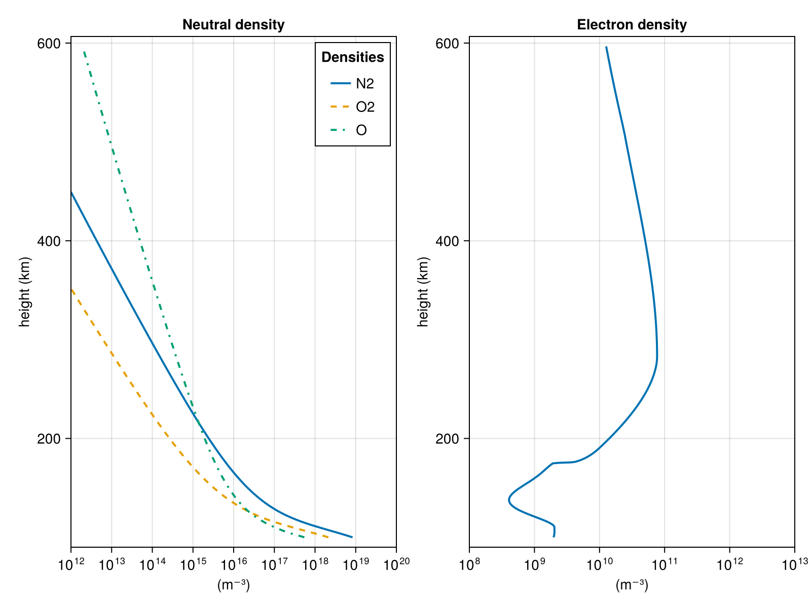
Energy levels
Excitation thresholds (vibrational, rotational, electronic, and ionization) for each neutral species.
figs[:energy_levels]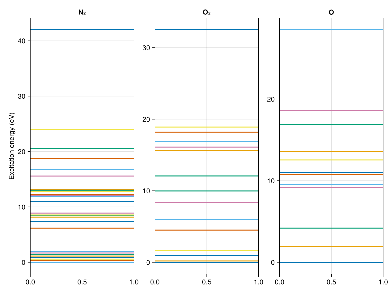
Energy grid
Variation of the energy bin width with energy. The grid is finer at low energies and coarser at high energies.
figs[:energy_grid]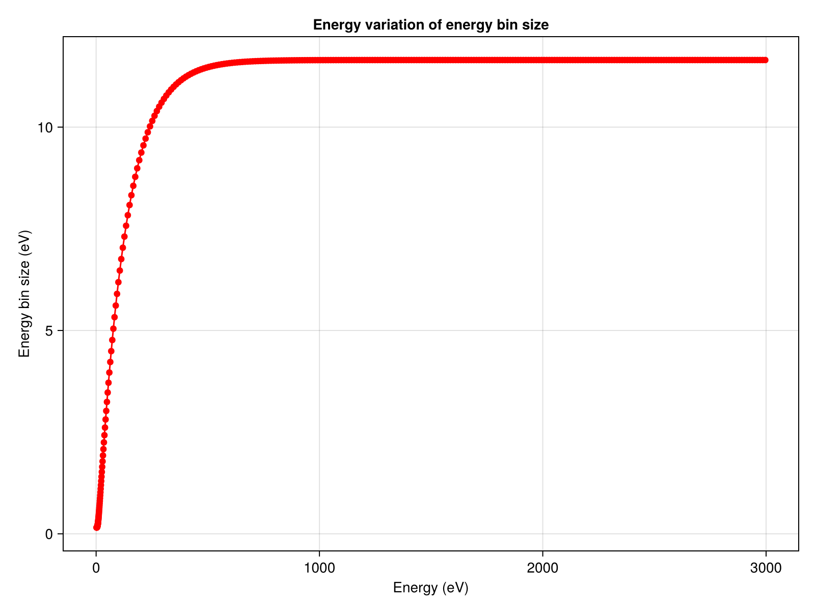
Cross-sections
Electron-impact cross-sections for all excited/ionized states of N₂, O₂, and O. Solid lines are excitation states and dashed lines are ionization states. Rotational/vibrational excitations are plotted with thinner lines.
figs[:cross_sections]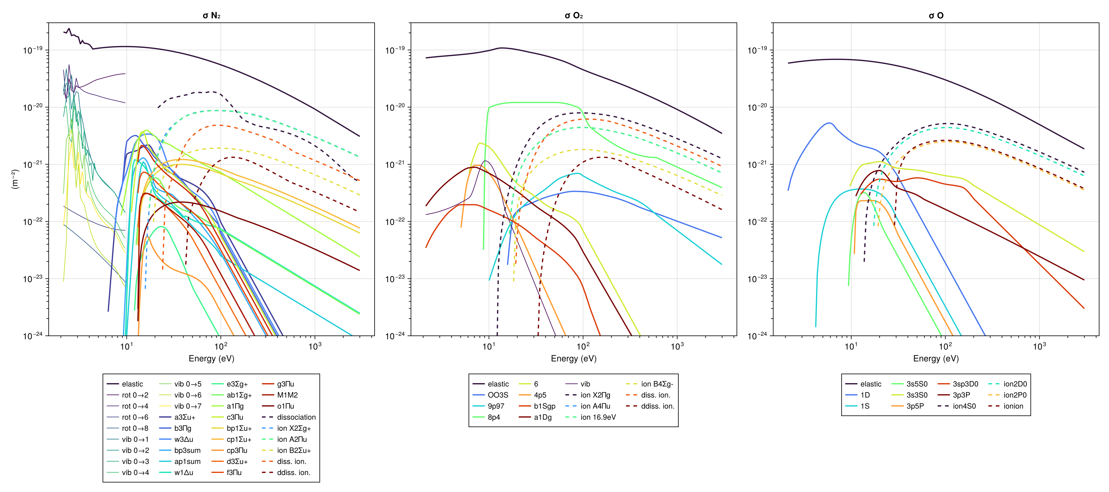
Phase functions
The scattering phase functions (elastic and inelastic) show, for each species, the probability distribution for scattering angles as a function of energy.
figs[:phase_functions]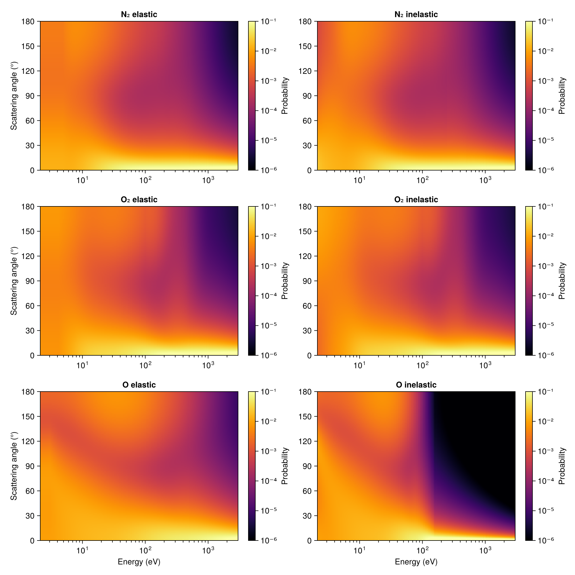
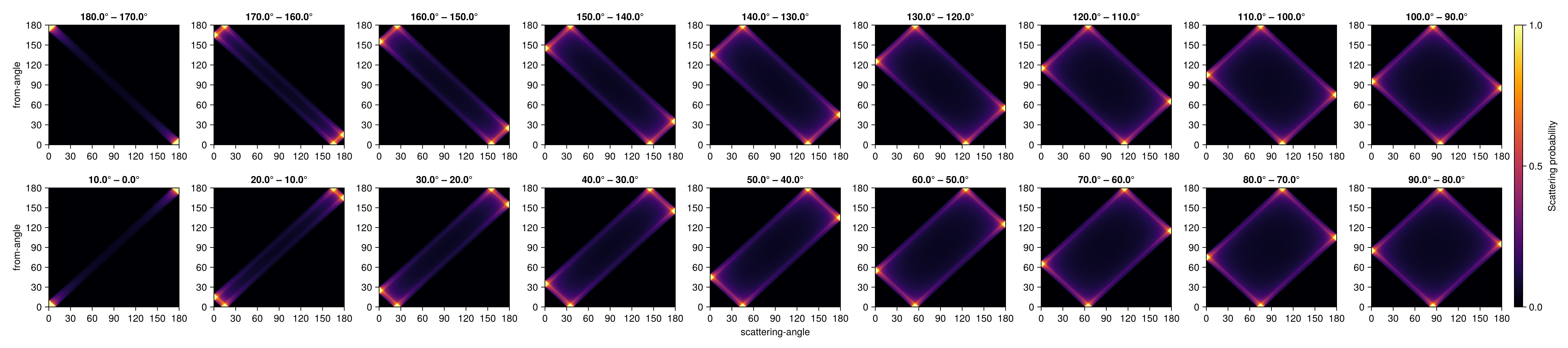
Scattering matrices
Pitch-angle transition probability matrices for each pitch-angle stream. Each panel shows the probability that an electron with an initial pitch-angle "from-angle" will end up in the stream/beam corresponding to the panel, after scattering with an angle "scattering-angle".
figs[:scattering]