Steady-State Simulation
AURORA can also run steady-state simulations. In this mode, it computes the final equilibrium electron distribution for a constant (time-independent) precipitating input. This is useful when you only care about the long-term response and don't need to resolve the precise temporal dynamics.
Setup
using AURORA

# Atmospheric model — default VISIONS-2 conditions
msis_file = find_msis_file()
iri_file  = find_iri_file()

model = AuroraModel(
    [100, 600],    # altitude limits [km]
    180:-15:0,     # pitch-angle bin edges [°]
    3000,          # maximum energy [eV]
    msis_file,
    iri_file,
    13             # magnetic field angle to zenith [°]
)
AuroraModel (not initialized):
├── AltitudeGrid(100.0 - 600.0 km, 410 points)
├── EnergyGrid(2.05 - 3002.16 eV, 336 bins)
├── PitchAngleGrid(12 beams)
├── ScatteringData: (not initialized)
├── Ionosphere(410 altitudes)
├── Species: N2, O2, O
└── B angle to zenith: 13.0°Maxwellian input spectrum
A MaxwellianSpectrum provides a smooth, physically motivated energy distribution set by a characteristic energy (formula from the Meier et al. 1989 paper):
flux = InputFlux(
    MaxwellianSpectrum(1e-3, 1000.0);  # 1 mW/m², characteristic energy 1 keV
    beams=1:2                          # two most field-aligned downward beams
)
InputFlux:
├── Spectrum: MaxwellianSpectrum(IeE_tot=0.001 W/m², E₀=1000.0 eV + LET)
├── Modulation: ConstantModulation()
├── Beams: [1, 2]
└── Source altitude: top of ionosphereCreate and run the simulation
savedir = mkpath(joinpath("data", "steady_state_example"))

sim = AuroraSimulation(model, flux, savedir)
AuroraSimulation (Steady-state):
├── Model: AuroraModel(AltitudeGrid(100.0 - 600.0 km, 410 points), EnergyGrid(2.05 - 3002.16 eV, 336 bins), PitchAngleGrid(12 beams))
├── Flux: InputFlux(MaxwellianSpectrum(IeE_tot=0.001 W/m², E₀=1000.0 eV + LET), ConstantModulation(), beams=[1, 2])
├── Mode: SteadyStateMode()
├── Savedir: data/steady_state_example
├── Time: single-step
└── Cache: not initializedrun!(sim)[ Info: Starting single-step steady-state simulation...Post-process
As for time-dependent simulations, it is possible to compute derived quantities from the raw electron flux and save them alongside the simulation output:
make_Ie_top_file(sim)              # boundary condition (input flux applied at top)
make_volume_excitation_file(sim)   # volumetric excitation rates for optical emissions
make_column_excitation_file(sim)   # column-integrated excitation rates (steady-state scalar)
make_current_file(sim)             # field-aligned electron currents and energy fluxes
make_heating_rate_file(sim)        # electron heating rates
Top flux saved in data/steady_state_example/analysis/Ie_top.nc
Volume excitation rates saved in data/steady_state_example/analysis/volume_excitation.nc
Column excitation rates saved in data/steady_state_example/analysis/column_excitation.nc
Currents saved in data/steady_state_example/analysis/currents.nc
Heating rates saved in data/steady_state_example/analysis/heating_rate.ncreaddir(savedir)4-element Vector{String}:
"analysis"
"config.toml"
"inputs"
"simulation_data.nc"Visualize
AURORA.jl provides helper plotting functions through a Makie extension. Install and load a Makie backend to access them (more information in Visualization).
Input flux
plot_input can be used to inspect the prescribed input spectrum directly from the simulation object:
using CairoMakie

fig = plot_input(sim)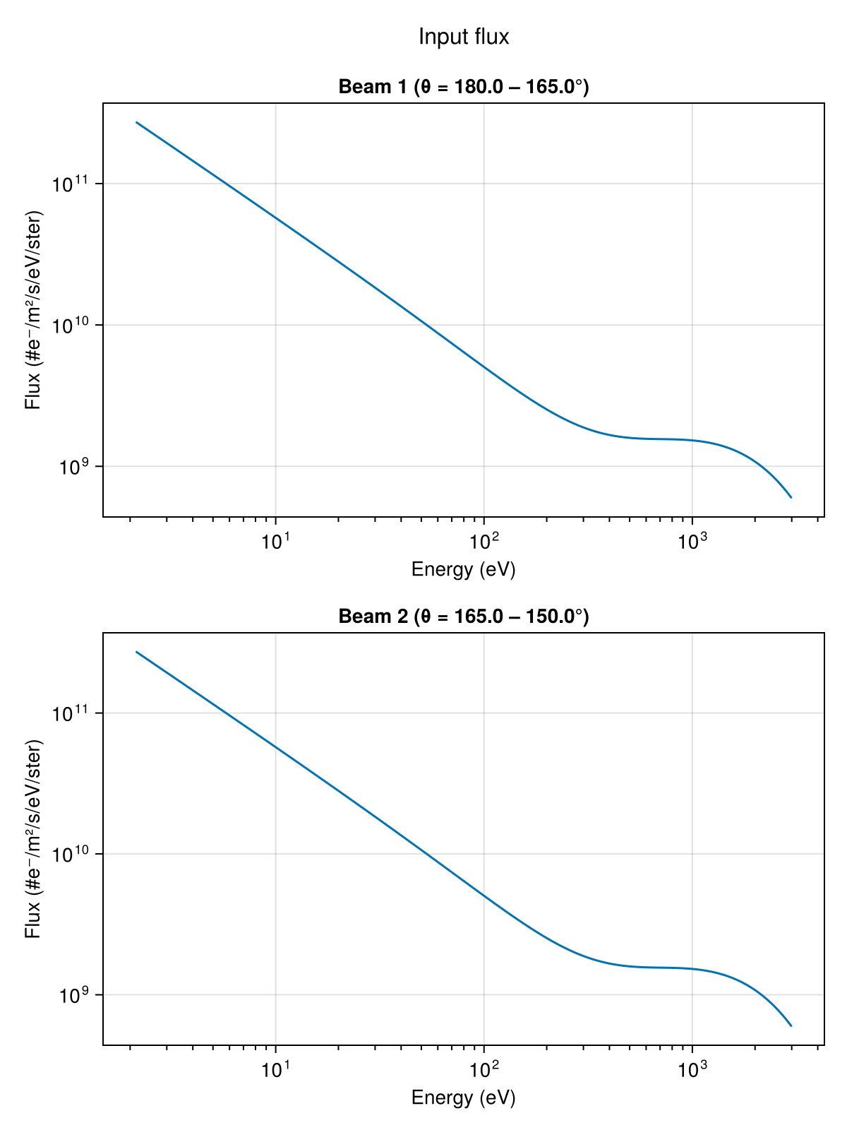
Volume excitation profile
plot_excitation! can be used to visualize the altitude profile of the volume excitation rate for a given emission line.
using CairoMakie
vol = load_volume_excitation(savedir)

fig = Figure()
ax  = Axis(fig[1, 1];
           xlabel = "Volume emission rate (photons/m³/s)",
           ylabel = "Altitude (km)",
           xscale = log10,
           title = "4278 Å")
plot_excitation!(ax, vol; field = :Q4278)
fig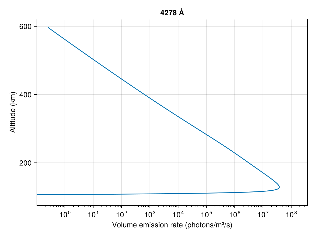
Next steps
- Time-Dependent Simulation — run the general time-dependent case.
- Input flux — explore all spectrum and modulation types.
- Post-processing & analysis — detailed walkthrough of all analysis functions.